Playing Enduro using a DQN Agent

Work does not have to be non-stop all the time. At Queryclick we are lucky enough to be encouraged to use personal development time to work on things not related to our daily job. During the last few weeks, I was looking into creating a Deep Q-Network (DQN) agent that is able to play the Atari game of Enduro.

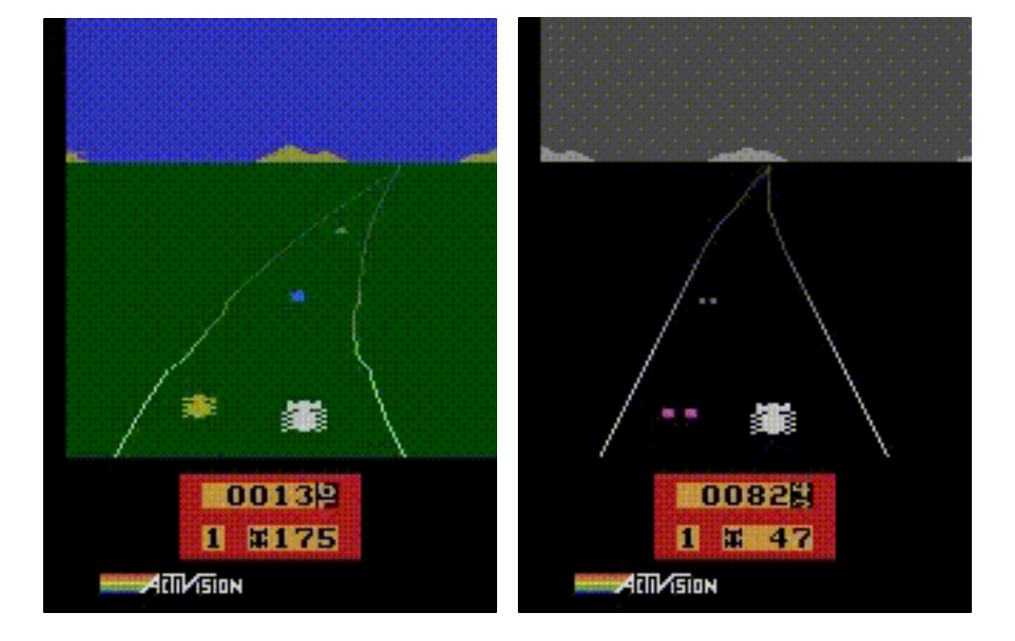
If you’re not familiar with Enduro this is a 1983 Atari 2600 racing game where the objective is to overtake at least a certain number of cars every game day to pass to the next day. The game introduced a few concepts still new at the time. These include day and night cycles, fog, snow and perspective.

In this article, I will explain how I set up this DQN agent, following the work from Mnih et al. in Human-Level Control through Deep Reinforcement Learning. We will follow the concepts introduced in this paper and get our own agent working and beating the game Enduro. I will at times deviate from this paper, things that make it easier to build, quicker to train, or changes that help us train this network on our own machine rather than workstation-level GPUs. We’ll be building the network in Pytorch. However, it can easily be built-in TensorFlow or otherwise. We will try to keep all the code modular so swapping different pieces will be possible if needed.

I will assume that you have a certain prior knowledge of reinforcement learning. Such as the basics, how the Q-learning helps an agent learn, function approximation, and epsilon-greedy to satisfy the exploration-exploitation dilemma.

This article will contain interesting snippets but will miss parts of the code that are just either boiler-plate or uninteresting. However, all the code is available in this GitHub repo, so feel free to read, clone, fork, PR, all are welcome.

Without further ado, let’s buckle up and begin.

Introduction

The OpenAI Gym was developed to standardize reinforcement learning environments. The collection has many different environments from Atari games, to bipedal walkers and other classical control problems. All environments have a step function which is passed an action, which will return the resulting state, a reward, whether the terminal state has been reached and other information in a dictionary. This is shown below.

The aim of the agent is to learn the appropriate action to pass to this step function depending on the previous state (and all the other states before it) and rewards.

The agent that we will use, DQN, is a type of model-free reinforcement off-policy learning agent, that without any knowledge of the environment, just plays the game, and learns as it goes. The inputs are the raw pixels from the Atari Gym which are then fed to a neural network. The network serves as a representation of how good it is to be in a particular state and which is the best action to take, ie. the action-value function. The agent can then use that action-value function to make its decisions.

Learning will be based on the Q-learning equation given in below:

$$Q(s_t,a_t)=Q(s_t,a_t)+\alpha\big[r_{t+1}+\gamma\max_aQ(s_{t+1},a_{t+1})-Q(s_t,a_t)\big]$$

Where the current action value (Q) updates are driven by the difference between the discounted max next action value (Q-next) and reward, and Q itself. This follows the principles of the Bellman equation. If the environment has few states and few actions, we can use a simple dictionary to save the combinations of all states and all actions, and the Q values corresponding to each combination. However, in this case, the state space is continuous and there are many actions that make this impossible due to memory limitations. Possibly yes we could discretize the state space, but that would limit our agent’s abilities. Therefore, we will use function approximation to represent the action value pairs, in this case, a neural network. It can be derived that the neural network change in weights needs to be driven by the equation below, where the gradient is calculated by our optimizer.

$$\Delta {\bf w}=\alpha(r_{t+1}+\gamma\max_a Q(s_{t+1},a_{t+1}, {\bf w})-Q(s_t,a_t,{\bf w})) \nabla_t Q(s_t,a_t, {\bf w})$$

If we train the network while playing naively, this will be unstable and diverge rather than converge to the correct value function. In their paper, Mnih et al. explain the reasons for this. These are mainly due to:

The samples being related to each other since the agent would be training online, hence them not being Independent and identically distributed (IID) as required by neural networks,
The learning process is constantly following a moving target which makes it difficult for the optimization to converge.

To help convergence, we will apply two techniques mentioned in the paper. These are:

Use a replay memory to sample unrelated samples rather than training on current samples.
Use two separate networks - an evaluation and target networks, and only update the target network once every $f$ times so that they are disjoint enough, that they don’t become unstable.

In addition to this, we also need to do some minor modifications to our environment to conform to the paper methodology. These help the model train and be more efficient. We’ll be:

Repeating the same action 4 times rather than taking an action every frame, and the max pixel value of the last two frames to avoid jitter.
Changing from an RGB input to a grey scale input
Resizing to an 84 by 84 image and scale to 0 to 255
Stack 4 latest frames as the output

Having covered all the features needed, let’s dive into the code. The flowchart below explains what we’ll be going for.

DQN Agent class structure

Environment modification

As explained above we need to do a few modifications to the OpenAI environment to be true to the paper and for the processing to be feasible. Two of the changes can be found pre-coded in the gym.wrappers package. However, The repeat actions and taking the max of the latest couple frames class as well as the normalize and resize class we have to build ourselves. Technically, a ResizeObservation class is available, but I had some issues getting it to work. I found it easier to add the one line needed in my own class.

To create the classes we’ll inherit from gym.Wrapper for the RepeatActionInFramesTakeMaxOfTwo class and inherit from gym.ObservationWrapper for the NormResizeObservation class. The first super-class wraps the whole environment while the observation-related one handles just the err… observation.

In the code below the RepeatActionInFramesTakeMaxOfTwo class has a defined deque of size 2 which is used to keep the latest 2 frames. When the step function is called, the step is repeated self.repeat times, each iteration keeping the reward and pushing the observation to the queue. When returning we return the total reward and the maximum of the latest two frames, ie the only two items in the queue. A reset function is also needed to clear the queue and append the first observation.

The NormResizeObservation class is much simpler since we just need to manipulate the observation. In this class, we receive the environment and shape as the constructor inputs. The observation_space of the environment needs to be redefined since we’re now scaling it to be between zero and one rather than zero and 255. In the observation function, we’re just resizing using OpenCV, and scaling by dividing by the 255 max value.

With that done, we can import the rest of the functions to set our environment up. We will use the NoFrameSkip-v4 version of Enduro. This means that output will skip no frames and the actions will be deterministic. This will allow us to get higher scores. More information about the types of environments can be found here.

Each wrapper is fed into the environment itself as well as any other parameters if needed. Similar to how we created our classes. In the snippet, we see the vanilla environment is first fed into the RepeatActionInFramesTakeMaxOfTwo class, then transformed to greyscaled, resized, normalized and finally stacked into a 4-pack.

The environment should now output as needed. This should help us use a smaller network and hence train faster.

Replay Memory

As explained by Mnih et al., replay memory is needed to store past information so then we can sample uniformly when doing training. This is important to keep samples in the batch unrelated so the model can learn efficiently. As we play the game we append to the end of the queue, discarded the oldest if the queue is full. Then, on every iteration for training, we uniformly sample a batch of batch_size from queue to train the models.

There are many ways how we could have implemented this. We could:

Use numpy arrays for each state, action, reward, next state and done flags
Use a deque FIFO where we put in a tuple of samples
Use a numpy structured array and push in a tuple of samples.

In my case, I felt that option 1 had too many different NumPy arrays which make it difficult to insert and batch, while option 2 is difficult to sample uniformly since deque objects are not really made for sampling. Option 3 is a bit more of an advanced NumPy structure, but we love learning new things right? So we went for it. And it is a beauty.

For this class we just need three functions. The constructor, the save method and the sample method.

In the constructor, we just define the datatypes, field names, and shapes of our structured array. We also define a counter so we know what is the next insertion point into the array as well as the memory_size.

In the save method we just push to this structured array.

And finally, in the sampling method, we get a random batch and return the values as a tuple of columns since we do not use the items row by row by column by column. Unfortunately, we have to wrap the columns into an np.array due to something related to how the structured array saves data into memory and Pytorch not liking it. Wrapping the columns this way reallocates memory and makes the arrays Pytorch friendly.

And that should be it for the replay memory. It is simple and beautiful, yet does it’s job. For the full class please have a look at the repository here.

Deep Q-Network

This is the part. The brain of the agent. The function approximator will tell us what action to take if we land in a particular state. As explained before, the inputs of this neural network will be the grey-scale resized images of the OpenAI Atari Gym output, and given these, the agent will give us a value for each action. This value indicates how good it is to take the respective action in the scenario. Since the inputs are images, we’ll have a few convolutional layers as lower levels, which are then flattened and passed onto a couple of linear layers.

The class we’re building here will inherit from torch.nn.Module. This adds the needed functionality to train using Pytorch.

In the constructor of the network, we can define these with a few parameters similar to what is used in the paper. We shall also use an MSE loss function and an RMSprop optimizer. Also, remember to set a device and send the graph to the device to be ready for processing.

In the snippet above both get_device() and calculate_flattened_shape are class helper functions, more detail can be found in the repo.

Once we create the constructor, we can then define the forward function that will be used to propagate the data forward through the network. Here, we’re mainly passing the observation through the different layers with a rectified linear unit as a non-linearity.

We can do the loss definition and optimization step within the agent. However, i opted to add this into the network as a function where it just needs the target and value and it would handle, calculating loss, sending to device, backpropagating and stepping. This should make it a bit more modular and if we’d want to implement this in Tensorflow, we can swap everything and have the same names.

The network class doesn’t only have the three functions described above. It has a few more functions such as the to_tensor shown below, as well as functions to load weight, save weights and get the device.

Once again, the class is available in the repo, specifically this page.

DQN Agent

Finally, we have the agent itself. This agent is rather simple once you get the concepts around DQN.

We first define the evaluation and target networks and the experience replay objects. The target and evaluation networks are identical. The evaluation network will be used to calculate the current action-value based on the current states, while the target network will create the hypothetical one that runs on the next states. If we only update the target network every $f$ times, this would make sure the network doesn’t have a continuously moving target and can help it converge.

We then define a choose action method. Since we’re following an epsilon greedy action selection, we choose a random action if the random number is less than epsilon else choose an action based on the output of the evaluation network. This should help exploration of states which weren’t visited yet.

We then define a learn function that uses the weight update equation explained earlier, and the evaluation and target networks for the current and next action-values repectively.

On every learn step we call the replace_target_network. This function checks the step against the frequency and updates the networks if necessary.

In the last line of the learn function, we call the decrement_epsilon which essentially reduces the size of epsilon so eventually it would be small so the model can start capitalizing on actions it thinks are best rather than taking actions randomly.

The rest of the functions are helper or interface functions such as the sample the memory, load and save models and saving the experience in memory.

Running Script

Now, we just have to combine every thing and run it. I use the script shown below. Essentially, it is doing the gym environment changes, and then looping over for a number of games, until each game is done, taking an action specified by the agent and learning. We also have a few handy tips such as collection of scores for plotting, and saving the model if it is the best model out there.

Training

Unfortunately, training this agent will take time. This can range from minutes to hours, depending on the number of games defined and the type of GPU. On my Nvidia GTX 1060, it took around 5 hours for 200 games.

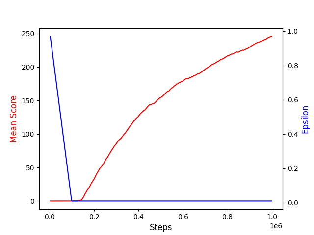
Once training is done, your plot should look something like this below which is good evidence of learning by the agent. The agent starts improving the score when the epsilon has dropped to the minimum value. This is expected, since the agent would then start acting greedily most of the time, taking the action that has the higher state-action value.

I have also attached a small gif below showing some cool overtaking by our DQN Agent. Look at it go! 🏎️

Obviously, there are still cases were it fails as shown below. However, it just recollects itself and tries again. A bit of what we should do when we ourselves hit a wall 😬

Conclusion

In this feature, we went through a few details on how to set up a DQN Agent to play the Atari game of Enduro. If you’re keen, you can also try this for the other Atari games too. Unfortunately, though, you cannot use this for any of the OpenAI gyms that has a continuous action space. For those types of models, a DQN won’t do and you’d have to use something similar to an actor-critic to perform policy optimization.

Once again feel free to access all the code. Any improvements are very welcome.